본 포스팅은 Universal Source-free Domain Adaptation논문의 리뷰를 다루고 있습니다.
개인적 고찰은 파란색으로 작성하였습니다. 해당 내용에 대한 토론을 환영합니다 :)
Motivation
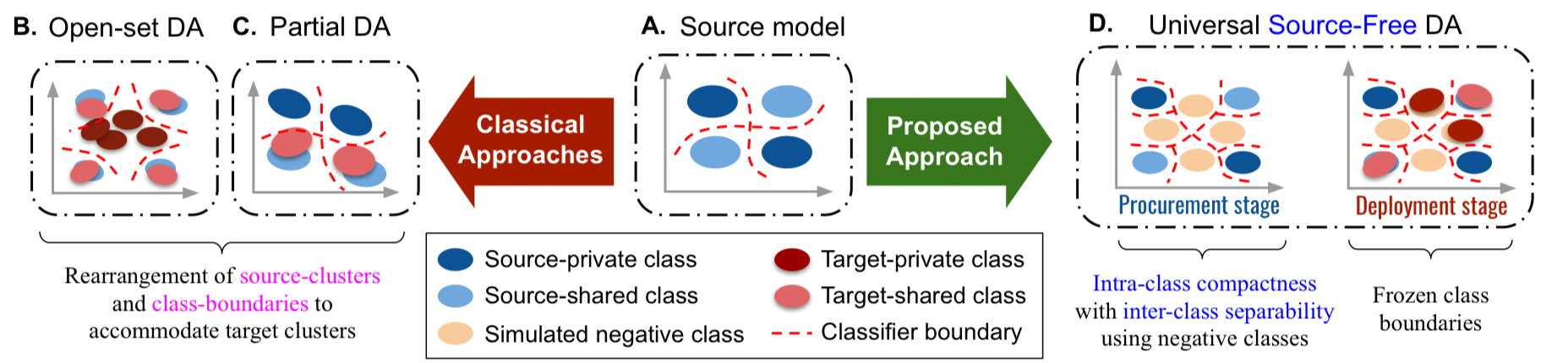
- Domain-shift가 있는 상황에서 knowledge of class-seperability (i.e., 학습된 classifier가 decision boundary를 긋는 능력―그냥 classification 성능)하는 많은 방법들이 존재하나, 이는 모두 source- target label-set relationship에 의존한 결과들임 (e.g. closed-set, open-set, partial-DA)
- 또한, 모든 unsupervised domain adaptation분야에서선 source와 target sample이 동시에 존재한다는 전제도 깔고 있음
- 본 논문에서는 이러한 impractical한 assumption들을 넣어서 domain adaptation을 하는 방법론을 제안하였음
- 보다 practical한 상황은 universal한 source-target 관계를 상정하고(즉, 어떤 relationship인지도 모르며 심지어 target domain이 하나가 아닐 수도 있음), target adaptation 시 source-free한 상황이여야 함
Background
- Category-gap (= label-set relationship)

- Universal―다중 target domain이 source domain과 다양한 관계로 뒤얽혀 있는 것 (하지만, 어떤 관계인지 모름 = 너무 많아서 다 고려하기 힘듦)
- Category-gap 별 접근 가능한 정보에 대한 모식도


Problem (keyword)
- Unsupervised domain adaptation (labeled → unlabeled)
- Universal
- Source-free
- Over-generalization
- fully-discriminative deep network는 training set이 커버하지 않는 영역까지 over-generalization하는 경향이 있음
- 이는, negative sample에 대해서도 highly confidnet하게 predict을 할 수 있다는 것을 의미함
- negative sample을 형성하더라도 모델이 이를 잘 학습할 수 있다는 것을 의미하며, 동시에 negative sample을 잘 만드는 것이 중요하다고 할 수 있음
Introduction
Term
- 방법론을 이해하기 앞서, source domain에는 source domain에만 존재하는 class와 target과 share된 class가 존재할 수 있음
- 이를 각각 source-private / source-shared class라고 함
- 마찬가지로 target에서도 target-private / target-shared class가 존재함
Pre-assumption
<논문의 핵심 Hypothesis>
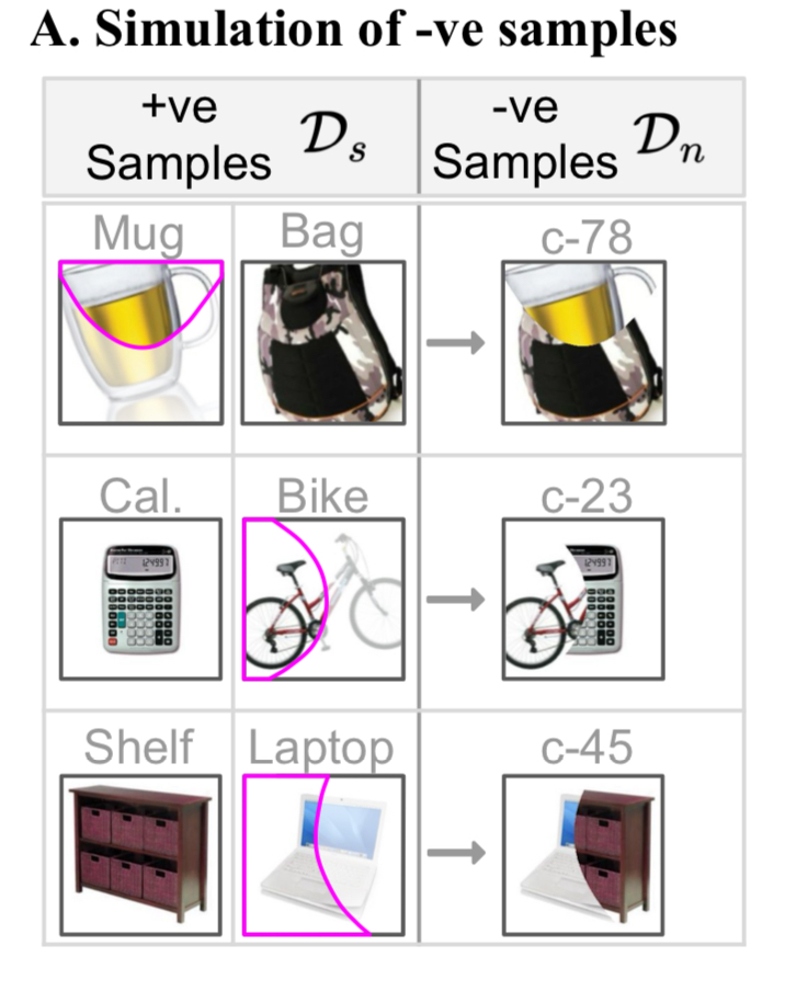
We hypothesize that the target samples have similar local part-based feature as found in the source data.
image data domain에서는 "어떤 image의 feature가 다른 image의 feature와 유사한 부분이 있다"는 것을 시사함
Example

예를 들면, 위의 예시에서 source dataset에 존재하는 해마와 호랑이의 이미지를 통해 target-private image에 해당하는 기린의 이미지를 형성할 수 있음 (해마의 몸통과 기린의 목이 pixel상에서 대각으로 긴 부분을 차지하므로 이를 비슷한 feature라고도 생각할 수 있음)
source-free domain adaptation에서 바로 이 사실을 이용해보면, 개념적으로 아래의 process처럼 생각해볼 수 있음
1️⃣ 해마와 호랑이를 합친 새로운 이미지를 정의함 → Composite image를 생성, Hypothetical class를 임의로 정의 (호마? 해랑이?)
2️⃣ source domain에서 source class들과 이 새롭게 정의한 class를 구분하도록 classifier를 만듦
3️⃣ 새롭게 정의한 class가 target-private images (즉, source와 공유되지 않는, target에서만 있는 image)를 분류하게 할 수 있음
Preview
- 그렇다면, 위 가설을 통해 source data를 이용할 수 없는 상황(source-free)에서, source class-seperability를 어떻게 target domain에서 working하도록 adaptation할 수 있을까?
- 심지어, source-target의 label-set relationship이 어떠한 지 조차도 모름 ― Universal
- Solution
- Target domain에서 source dataset에 대한 정보 access없이 (source-free) target class-seperability를 얻고 싶음
- target-shared class들은 source-shared class들과 잘 mapping이 될 수 있으니 어찌저찌하면 되는데, 문제는 target-private class들임
- 이러한 target-private class들을 잘 구분해내기 위해서 source data를 동해 hypothesis class를 만들고 이것이 target-private class의 feature를 잘 표현하도록 기대하는 것임
Method
본 논문에서는 1) Procurement stage와 2) Deployment stage를 두어 해결하고자 하였음
(각각 negative image를 합성하는 단계, 실질적인 adaptation을 진행하는 단계)
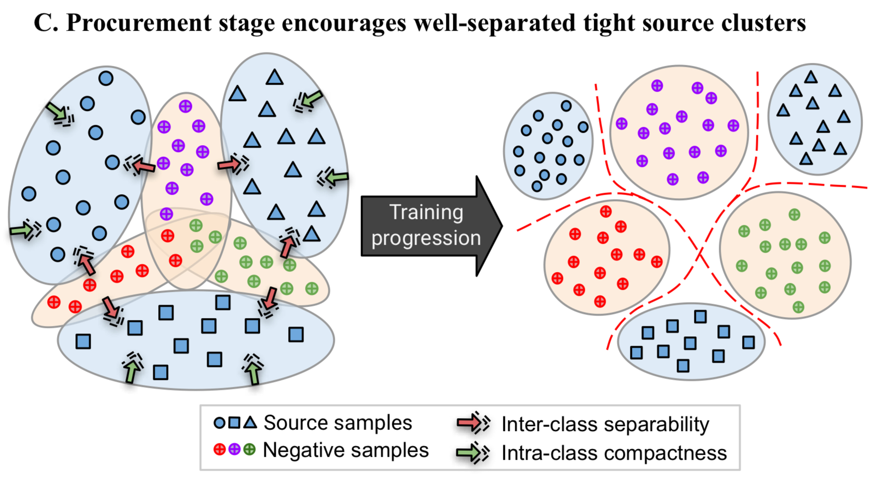
Stage 1. Procurement
위 아이디어를 실현하기 위해선, negative sample을 잘 만드는 것이 중요함
- 합성된 이미지는 기존 class들과 전혀 다른 이미지는 아니어야 함 (합성된 이미지가 new domain을 개척하지 않아야 함)
- source domain에서 inter-class seperability와 intra-class compactness를 모두 증가시켜야 함
- 우려할 수 있는 사항은, composite image의 softmax probability가 원본 이미지들 image class에서 높게 할당될 수 있음
- 또한, 단순 mixup이나 adversarial noise를 이용하여 새로운 이미지를 형성하는 것은 source domain이 아니라 새로운 domain을 개척하는 일이 될 수 있음
- 그리하여 위의 오른쪽 이미지처럼 local part feature를 더하여 합성해야 함 (Key : source-target의 shared feature를 local part related feature로 정의하였기 때문에, 이미지 합성법도 이 가정에 근거해야 함)
- local part related feature : 해마의 몸통 = 기린의 목 = "길다"
Stage 2. Deployment
- 결국, source-free한 상황에서 source의 negative sample과 target-private class를 adaptation하는 것이 중요함
- 또 하나의 중요한 사실은 target domain에서는 label이 없는데, 이를 어떻게 학습해야할까?
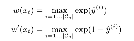
(a) Source Similarity Metric (=pseudo label)
- 먼저, target domain에서 label 역할을 하는 source similarity metric (SSM)을 정의함 (label이 없는 target domain에서 pseudo-label역할)
- 정의한 SSM은 기능적으로, 높은 값을 가질수록 source의 positive class와 유사하다는 것이고 (동시에, label common space의 class와도 가까워야함)
- 낮은 값을 가질수록 source의 negative class와 유사하다는 것(동시에, target private class와도 가까워야함)으로 design되어야 함
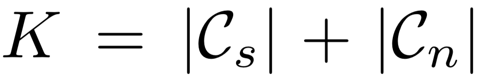
SSM을 $w(x)$로 정의할 때, 각 source / target별 class종류에 따른 SSM의 순서는 다음과 같아야 함
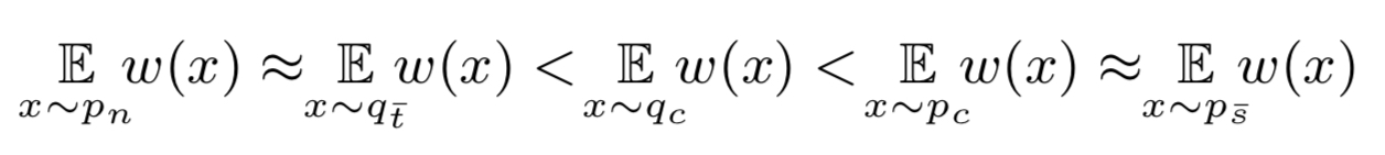
(bar notation은 private, p는 source, q는 target 분포
$\bar{s}$는 source-private, $\bar{t}$는 target-private, c는 common label space를 의미함)
$w(x)$는 $x_t$를 source model에 통과시켜 도출된 logit에 softmax를 취한 output이어야 하는데 (class prediction probabiliity) 본래, negative class까지 합친 차원의 vector이나 source positive class에 대한 것만으로 정의함
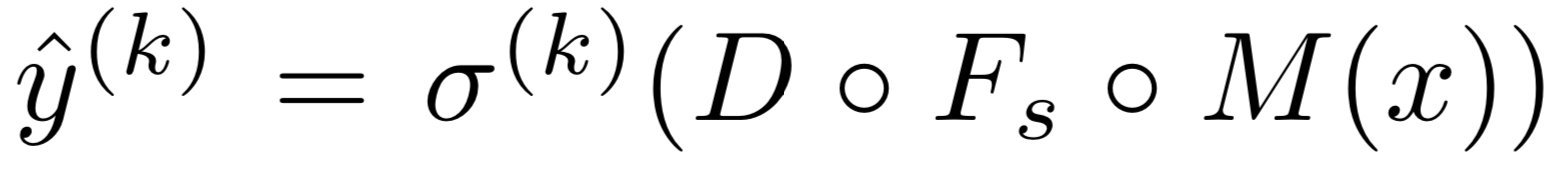
(M은 backbone, $F_s$는 source feature extractor, D는 classifier, $\sigma$는 softmax function)
(b) Source-free domain adaptation
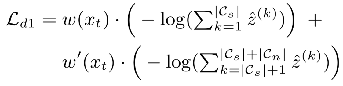
- 위 SSM을 label삼아 target network를 학습시키는데,
높은 SSM일수록 source positive와 가깝게 학습이 되고,
낮은 SSM일수록 source negative와 가깝게 학습이 되게 해야함 -> cross entropy개념
- target network를 다음과 같이 정의할 때,

- target network로부터 도출된 softmax prediction 는
$$ \hat{z}^{(k)} = \sigma^{(k)}(h)$$
- 하지만, 여기서 의문이 드는 것은 과연 아무리 source negative image가 target image의 feature를 나타낼 수 있다하더라도 다른 domain의 label로 학습하는게 working하는가?
- label information이 없는 target domain에서는 target softmax prediction에 uncertainty가 존재할 수 있음
- 본 논문에서는 이를 entropy minimization으로 해결하고자 함

- 정리하자면, Deployment단계에서는 pseudo-label을 통해 target network를 학습시키고 target network가 제대로 된 softmax prediction을 뽑아내도록 uncertainty minimization(=entropy minimization)을 동시에 수행함
- The final loss, $\mathcal{L}_d$는,
$$ \mathcal{L}_d = \mathcal{L}_{d1} + \beta\mathcal{L}_{d2} $$
($\beta$ : entropy minimization의 importance를 조절하는 hyperparameter)
Architecture
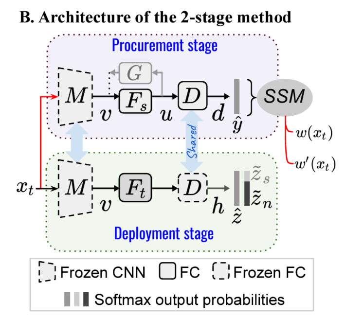
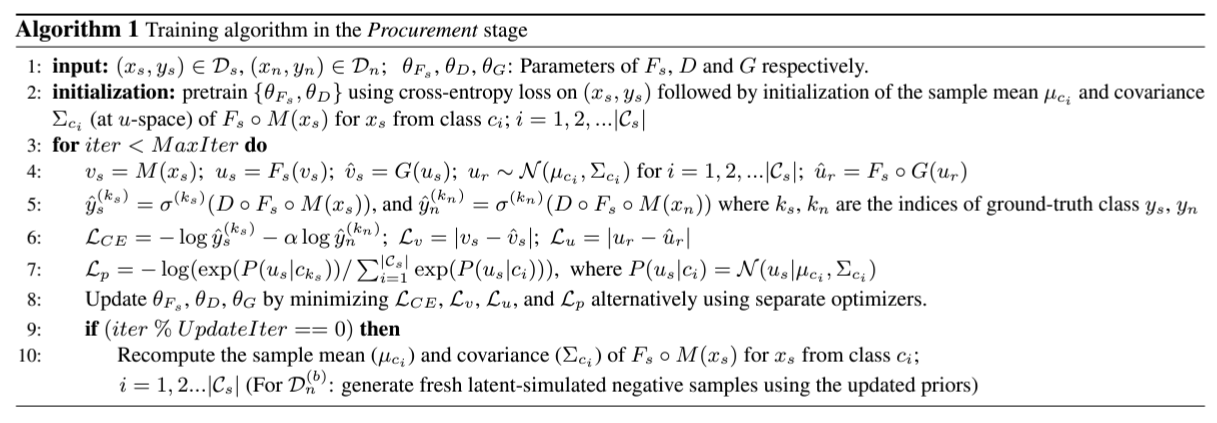
- 본 논문의 핵심은 Procurement stage에 있음 → Procurement stage를 잘해야 deployment stage에서도 learning이 잘 된다고 할 수 있음
- Procurement stage에서의 관건은 source domain 내에서 새로은 domain을 개척하지 않고 source domain class cluster사이에 분포하는 negative sample을 만드는 것임
- souce positive class들의 extracted feature들에 대해서 prior분포를 정의 (즉, feature space에서의 prior distribution을 정의함)

- 위 분포를 정교화하여 high inter-class seperability & high intra-class compactness하도록 함 ($L_p$와 Algorithm 1의 line 9~10)
- 위 Procurement stage 알고리즘에는 총 4개의 loss와 distribution parameter update가 있음
- $L_{CE}$ : source positive class와 생성된 negative class를 각각 구분하도록 학습하는 cross-entropy loss → update $\theta_{Fs}$, $\theta_{D}$
- $L_{p}$ : the positive source class의 feature space의 분포 likelihood를 maximize → update
- $L_{v}$ : v를 정교화, $|v_s - G(u_s)|$ → update $\theta_{G}$
- $L_{u}$ : u를 정교화, $|u_r - Fs \circ G(u_r)|$ → update $\theta_{G}$, $\theta_{Fs}$
- Procurement stage에서 잘 정립된 분포 cluster들이 Deployment stage에서 흩뜨려지지 않아야 함
- 이에, domain specific feature extractor를 각각 두고, $F_t$를 $F_s$로 initialize함


